Self-study

Code

try:
    import fysisk_biokemi
    print("Already installed")
except ImportError:
    %pip install -q "fysisk_biokemi[colab] @ git+https://github.com/au-mbg/fysisk-biokemi.git"

Code

import numpy as np

1 Python as a calculator

We can use Jupyter notebooks as a calculator with all the operations we are familiar with from a regular calculator.

1 + 1       # Addition with +
3 - 1       # Subtraction with - 
4 * 4       # Multiplication with *
20 / 5      # Division with /

(a) Doing some calculations

Use Jupyter notebook to calculate the following:

\(21 + 21\)
\(53 - 11\)
\(6 \times 7\)
\(\frac{546}{13}\)

# Write your code in this cell

(b) Using variables

As also mentioned in “Introduction to the molecules of life”, it is often helpful to define quantities in variables, which gives them a name that can be used later. A variable is defined by using =, for example, we can define

a = 21 + 21

This means that the result of the calculation is stored in a.

Repeat the calculations from exercise 1, but now save each result in a variable

a = 21 + 21 
b = ... # Replace ... with your code
# Create variables c and d.

We can then use the defined variables in a new calculation

total = (a + b + c + d) / 4
print(total)

42.0

(c) A biological calculation

In “Introduction to the molecules of life” we have made calculations about the number of cells in different parts of the body.

total_cells = 37_000_000_000_000
brain_cells = 86_000_000_000
liver_cells = 240_000_000_000
skin_cells = 1_600_000_000_000

Use Jupyter as a calculator to calculate the percentage each category represents of the total number of cells in the body, i.e., for each category calculate

\[ P = \frac{\mathrm{Number}}{\mathrm{Total}} \times 100 \]

brain_pct = ... # Replace ... with your code.
liver_pct = ... # Replace ... with your code.
# Calculate and create variable for skin_pct

print(brain_pct)
print(liver_pct)
print(skin_pct)

0.23243243243243245
0.6486486486486486
4.324324324324325

(d) Using functions

Note

When we perform the same calculation multiple times, it’s smart not to have to write the same code again, it makes the code more readable and reduces the chance of making errors. The way to avoid this is by using functions, a function in Python defines a recipe that is executed when it is called.

Above, we have for example used the function print to write output. A function is defined like this

def my_function(a, b):
    result = a * b 
    return result

It’s important that the function is indented (pushed to the right) as Python needs this to read it. When a function is defined as above, the calculation is not performed, just like writing down a recipe doesn’t make a meal, only when the function is “called” is it executed

my_function(6, 7) # Would give 6*7 = 42

Complete the function below so it calculates the percentage of value out of total.

def percentage(value, total):
    result = ... # Replace ... with your code.
    return result

We can then use the function to calculate the percentages

brain_pct = percentage(brain_cells, total_cells)
liver_pct = percentage(liver_cells, total_cells)
skin_pct = percentage(skin_cells, total_cells)
print(brain_pct, liver_pct, skin_pct)

0.23243243243243245 0.6486486486486486 4.324324324324325

(f) Special functions

Note

We have now seen that we can use Jupyter notebooks as a calculator to make calculations with the basic arithmetic operations. However, we often need to calculate power functions, square roots, exponential functions or logarithms.

Fortunately, this is also easy with Python, as we can use a package that implements these operations as functions - specifically numpy.

Power functions, i.e., \(x^k\) can be calculated as

x**k

The other three can be calculated with NumPy as

np.sqrt
np.exp
np.log

Use numpy functions to calculate the following

\(6.4807^2\)
\(\sqrt{1764}\)
\(e^{3.737669}\)
\(\log{(66.6863)}\)

import numpy as np # This imports NumPy so we can use the functions.

result_1 = ... # Your code here
result_2 = ... # Your code here
result_3 = ... # Your code here
result_4 = ... # Your code here

print(result_1, result_2, result_3, result_4)

Code

import numpy as np

2 Functions & arrays

Previously we looked at functions, we will build on that now. Remember that a function is a recipe that describes how a calculation should be performed that can be reused many times.

A function is defined with def followed by its name and its parameters (also called arguments) are placed in the parentheses.

def my_function(a, b):
    result = a * b 
    return result

The function is only executed when it is called, in this case for example

my_result = my_function(6, 7)
print(my_result)

Where we now have the output of the function in the variable my_result.

(a) Calculaling cell sizes

The tables below show the radius of different cell types

Cell sizes
Cell type	Radius
Mycoplasma	~0.2–0.3 µm
Typical bacterium	~1–2 µm
Yeast cell (S. cerevisiae)	~5–7 µm
Red blood cells (human)	~7–8 µm
Lymphocyte (white blood cell)	~8–10 µm
Typical animal cell	~10–20 µm
Typical plant cell	~20–100 µm
Human egg cell (oocyte)	~120–140 µm
Neuron (cell body)	~10–100 µm

We have previously calculated the volume of the cells by assuming that they are spherical, whereby the volume is given by

\[ V(r) = \frac{4}{3}\pi r^3 \]

Write a function that takes radius r as an argument and calculates volume -
you can use np.pi instead of writing \(\pi\) yourself!

def ... # Replace with your code
    ... # Replace with your code

Call the function with some of the different radii from the table

mycoplasma_volume = ... # Replace with your code
print(mycoplasma_volume)
# Do the same for some of the other cell types
...

(b) Calculations with arrays.

Note

We have previously seen some of the different data types in Python

Integers int
Floats float
Strings str

But there are many other types that can be helpful in different contexts. One such type is numpy arrays, an example of a numpy array is shown below

A = np.array([1.0, 2.5, 3.5])

One of the smart things about arrays is that we can perform operations on all the content at once

B = 2 * A 
print(B)

[2. 5. 7.]

The same is true for using the array A in a function, for example we can write

def example_function(array):
    return 1 + array

print(example_function(A))

[2.  3.5 4.5]

Create an array that contains the specified cell radii and use your volume function to calculate the volume of all cells at once

radii = np.array([...]) # Replace ... with your code

cell_volumes = ... # Replace ... with your code.
print(cell_volumes)

(c) Array operations

Note

There are many other operations we can perform on arrays, such as finding the largest or smallest number

We can find the cell type with the largest volume as

np.max(cell_volumes)

np.float64(9202772.0799157)

The corresponding function for finding the smallest number is called np.min.

The cell below creates an array with 1000 numbers

array_with_numbers = np.random.rand(1000) * np.exp(3.737669)

Use np.max to find the largest number in array_with_numbers

largest_number = ... # Replace ... with your code
print(largest_number)

(d) Array indexing

Note

Sometimes we are interested in specific entries in an array, so we also need to be able to extract data from an array. This is “indexing”, for example if we have an array

my_array = np.array([0, 2, 4, 6, 8, 10, 12, 14, 16, 18, 20])

We can extract the fourth number like this

fourth_number = my_array[3]

In Python we start counting from 0, so the fourth number is found at position 3.

Use indexing to calculate the sum of

The last number (Position 10)
The second number (Position 1)
The fourth number (Position ??)
The eighth number (Position ??)

sum_of_numbers = ... # Replace with your code
print(sum_of_numbers)

(f) Working with data

In molecular biology we often work with spectra, where the axes are for example

\(x\): Wavelength measured in nm
\(y\): Absorption coefficient

from fysisk_biokemi import load_dataset

df = load_dataset("chlorophyll")
print(df)

wavelengths = df['Wavelength(nm)'] # An array with 501 entries
absorption = df['AdsorptionCoefficient'] # An array with 501 entries

     Wavelength(nm)  AdsorptionCoefficient
0               300              20487.000
1               301              20547.000
2               302              20642.000
3               303              20767.000
4               304              20899.000
..              ...                    ...
496             796                 26.665
497             797                 15.556
498             798                 29.164
499             799                 21.473
500             800                 18.396

[501 rows x 2 columns]

import matplotlib.pyplot as plt 
fig, ax = plt.subplots()
ax.plot(wavelengths, absorption)
ax.set_xlabel('Wavelength [nm]')
ax.set_ylabel('Absorption Coefficient')

Text(0, 0.5, 'Absorption Coefficient')

Caution

How the plotting works with be explained in another exercise, for now just appreciate the pretty plot.

We want to use NumPy to find what the maximum absorption coefficient is, and at which wavelength it occurs.

Start by finding the maximum absorption coefficient using np.max

max_absorption = ... # Replace ... with your code
print(max_absorption)

We can use another function from NumPy to find the wavelength where the absorption coefficient has its maximum

index_max_abs = np.argmax(absorption)

Note

np.argmax finds the index of the argument that contains the max value.

Now use index_max_abs to extract the corresponding wavelength from wavelengths

wavelength_max_abs = ... # Your code here

import matplotlib.pyplot as plt 
fig, ax = plt.subplots()
ax.plot(wavelengths, absorption)
ax.axvline(wavelength_max_abs, color='red')
ax.set_xlabel('Wavelength [nm]')
ax.set_ylabel('Absorption Coefficient')
plt.show()

3 Parentheses

Later in the course we will see equations such as the quadratic binding equation

\[ \theta = \frac{K_D + [P_{tot}] + [L_{tot}]}{2[P_{tot}]} - \sqrt{\left(\frac{K_D + [P_{tot}] + [L_{tot}]}{2[P_{tot}]}\right)^2 - \frac{[L_{tot}]}{[P_{tot}]}}, \] which can be used to describe titration data that reports protein saturation as a function of total ligand concentration.

Calculating this function requires that we are careful with parentheses! Which we have all learned, but since it is very important in this context, it is worth refreshing.

(a) Mind the \((...)\)

For the following pairs of expressions, calculate both (by hand or mentally, according to preference.)

\(2 + 3 \times 4\) vs. \((2 + 3) \times 4\)
\(10 - 2^2\) vs. \((10 - 2)^2\)
\(100 / 10 \times 2\) vs. \(100 / (10 \times 2)\)
\(\frac{12 + 8}{4}\) vs. \(12 + 8 / 4\)

(b) Beware of the \((...)\)

For the three calculations below, consider what the result is before you run the cell.

a = 1 + 2 * 3 ** 2

b = (1 + 2) * 3 ** 2

c = 1 + 2 * (3 ** 2)

The cell below prints the result for each calculation

print(f"{a = }")
print(f"{b = }")
print(f"{c = }")

(c) Fix the \((...)\)

We want to calculate the expression

\[ \frac{a + b}{c + d} \]

Someone has implemented the function below, but it is incorrect - your task is to fix it.

def function(a, b, c, d):
    return a + b / c + d

result_1 = function(152, 16, 2, 2)
print(result_1)

(d) Implement the \((...)\)

The first term of the quadratic binding equation is

\[ \frac{K_D + [P_{tot}] + [L_{tot}]}{2[P_{tot}]} = \frac{a + b + c}{2 b} \]

Complete the function below so it calculates this expression

def first_term(a, b, c):
    return ... # Replace ... with your code.

result = first_term(100, 2, 66)
print(result)

4 Working with datasets

Code

import numpy as np
import pandas as pd
from fysisk_biokemi import load_dataset, get_dataset_path
import matplotlib.pyplot as plt

We have previously looked at a dataset about the absorption spectrum of chlorophyll, but we weren’t focused on how we handled this dataset.

What we achieved was plotting the dataset, as seen below

chloro_df = load_dataset("chlorophyll")
wavelengths = chloro_df['Wavelength(nm)'] # An array with 501 entries
absorption = chloro_df['AdsorptionCoefficient'] # An array with 501 entries

fig, ax = plt.subplots()
ax.plot(wavelengths, absorption)
ax.set_xlabel('Wavelength [nm]')
ax.set_ylabel('Absorption coefficient')

Text(0, 0.5, 'Absorption coefficient')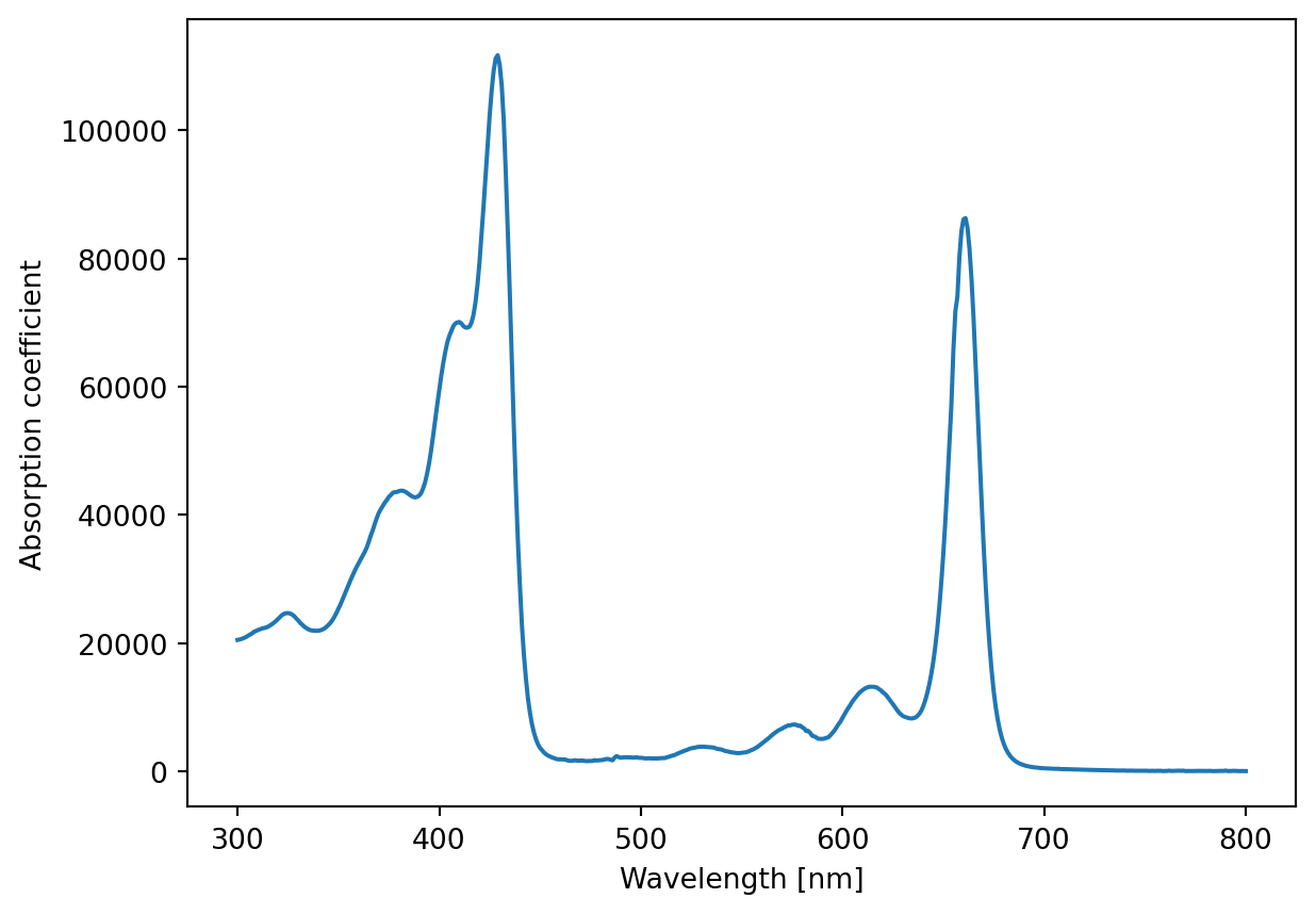

This time we will investigate a bit more how we can work with a dataset.

NumPy arrays as datasets.

It is important that we keep good track of our data, it is often smart to use a data type that helps us with this. We have previously seen arrays, which is one possibility - e.g.

a = np.array([1, 2, 3, 4])
b = np.array([1, 4, 9, 16])

But if we have many quantities it can quickly become unmanageable - another possibility is to store all our quantities in the same array

combined_array = np.array([[1, 2, 3, 4], [1, 4, 9, 16]])
print(combined_array[0, :]) # Corresponds to a
print(combined_array[1, :]) # Corresponds to b

[1 2 3 4]
[ 1  4  9 16]

Note

NumPy arrays can have multiple dimensions, combined_array here has two dimensions (like a matrix). In this case each row describes one of our quantities. Here : is used to mean “all” in indexing so [0, :] can be read as first row all columns.

But then we need to keep track of which axis contains which quantity. Sometimes it can be fine to keep our data as np.array but other times it’s better in other ways.

Pandas `DataFrame`

One such other way to handle a dataset is by using a new type, namely a pandas DataFrame.

We can create a DataFrame from our two arrays like this;

df = pd.DataFrame({"a": a, "b": b})
df.style.hide() # This just make printing a bit simpler
print(df)

Here we have three columns, the first is index, the second is a and the third is b.

Note

The chlorophyll dataset was actually also a DataFrame.

With a DataFrame we have more possibilities for indexing, we can for example use the name of the column.

print(df['a'])

0    1
1    2
2    3
3    4
Name: a, dtype: int64

(a) Calculations with a dataset

Calculate the formula \(2 \times a\) where \(a\) comes from the dataset above df

result = ... # Replace ... with your code.
print(result)

(b) Elementwise operations

We can also add two arrays together using whats called an elementwise operation where for example the first element of each array are added, the second elements are added and so on.

Use this to calculate \(c = a + b\).

c = ... # Replace ... with your code
print(c)

(c) Plotting a dataset

Make a plot of \(a\) versus \(b\) where the two quantities come from the DataFrame df.

fig, ax = plt.subplots()
... # Write your code to plot.

Tip

You need to extract the two columns df['a'] and df['b'] and put those in ax.plot(..., ...).

(d) Datasets from files

Note

Often we don’t want to write our dataset directly into code, but store them as separate files that could for example come from experimental equipment.

We can get data from an Excel file, like this

#| eval: false
dataset_path = "/path/to/the/file/that/has/our/data.xlsx"
df = pd.read_excel(dataset_path)

Through out the course we will use a widget to load datasets from your computer, this makes it a little easier to manage with Google Colab.

You can run the cell below and click on the “Upload”-button that appears and you use that to select the reverse_reaction.xlsx dataset that you can download from here datasets under the “Additional Datasets” tab at the bottom of the page.

You should save it somewhere where you can find it again - a good idea would be to put it in a folder specifically for this course.

from fysisk_biokemi.widgets import DataUploader
from IPython.display import display 
uploader = DataUploader()
uploader.display()

Once you’ve uploaded the dataset you can run the next cell

df = uploader.get_dataframe()
display(df)

Based on the information that has been printed out what do you think the dataset contains? Think about the following

How many columns are there?
What is the title of each column?
How many rows are there?

(f) Plot the dataset

Now that we have retrieved the dataset we want to investigate it more easily by plotting it.

Complete the code below

fig, ax = plt.subplots()
ax.plot(df['time'], ..., label='[A]') # Replace ... with your code
... # Replace ... with your code that plots time versus concentration_B 
ax.set_ylabel('Concentration') # Sets name on y-axis
ax.set_xlabel('Time') # Sets name on x-axis
ax.legend()# Shows what 'label' each plotted curve has.

What do you think the dataset shows?

(g) Calculation with dataset

As mentioned we can also do calculations with a dataset. Calculate \[ [T] = [A] + [B] \] And complete the plot in the cell below

concentration_T = ... # Replace ... with your code

fig, ax = plt.subplots()
ax.plot(..., ..., label='[T]', color='C2') # Replace both ... with your code.

# From before
ax.plot(df['time'], df['concentration_A'], label='[A]')
ax.plot(df['time'], df['concentration_B'], label='[B]')
ax.set_ylabel('Concentration') # Sets name on y-axis
ax.set_xlabel('Time') # Sets name on x-axis
ax.legend() # Shows what 'label' each plotted curve has.

Why do you think it looks like it does?

1 Python as a calculator

(a) Doing some calculations

(b) Using variables

(c) A biological calculation

(d) Using functions

(f) Special functions

2 Functions & arrays

(a) Calculaling cell sizes

(b) Calculations with arrays.

(c) Array operations

(d) Array indexing

(f) Working with data

3 Parentheses

(a) Mind the \((...)\)

(b) Beware of the \((...)\)

(c) Fix the \((...)\)

(d) Implement the \((...)\)

4 Working with datasets

NumPy arrays as datasets.

Pandas DataFrame

(a) Calculations with a dataset

(b) Elementwise operations

(c) Plotting a dataset

(d) Datasets from files

(f) Plot the dataset

(g) Calculation with dataset

Pandas `DataFrame`