Biomolecular visualization with PyMOL 3
1 Overview
This tutorial provides a basic introduction to molecular visualization with PyMOL 3. It only covers the use of the graphical user interface (GUI) and not the use of the command line. It covers aspects of the program useful for structural biology and medicinal chemistry such as exploring protein-ligand interactions, as well as making figures for use in reports.
1.1 The graphical user interface (GUI)
The PyMOL GUI consists of multiple panels as shown in Figure 1. The provides a set of handy buttons for quick access to various functions. The main display panel provides the visualization of the loaded molecules while the object panel on the right-hand side provides a menu of options for the loaded molecules. While the object menu provides various operations by clicking, the same tasks can be achieved using the command line located at the bottom of the window. The log window contains log of which commands have been executed and details of selections. Note also the of the object menu that contains controls for mouse, wizards, sequences and movies and a button to hide/show the log window.
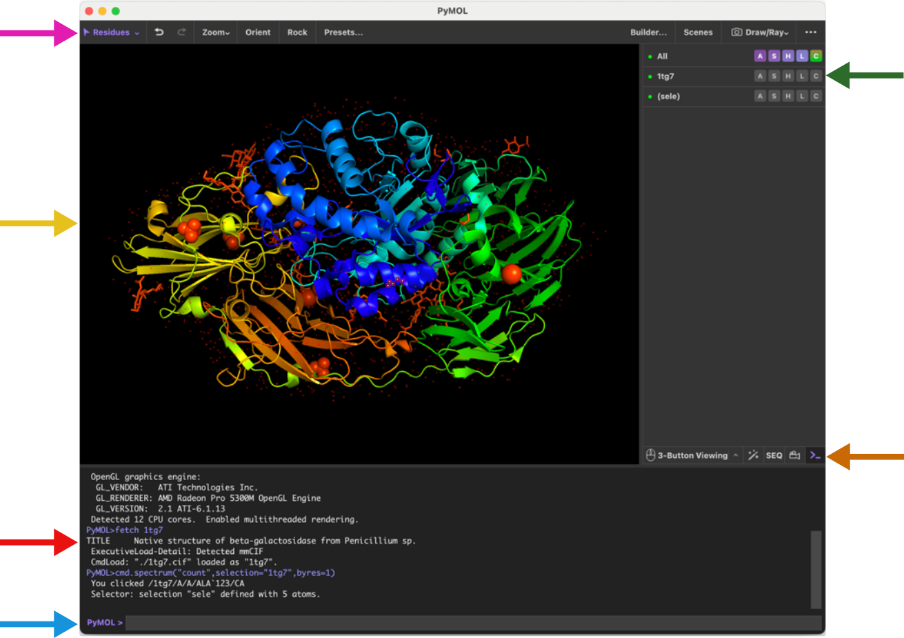
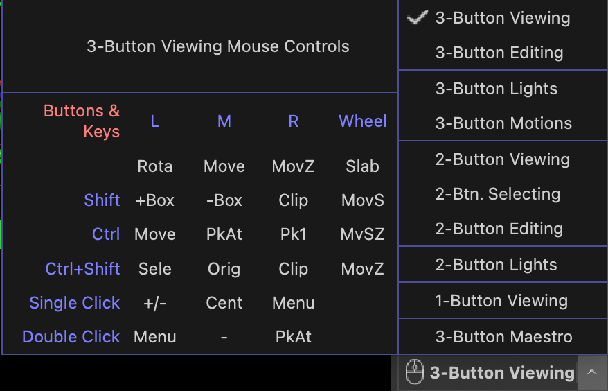
It is highly recommended to use a 3-button mouse for navigating PyMOL as the 3-button viewing mode is the most convenient and has most functionality attached. You can use the to set the mouse mode and see a guide to the different functions that are available (see figure below).
Most tasks in PyMOL can be achieved using the object panel on the right-hand side of the display panel. Here, each line (or entry) in the menu correspond to the objects you have loaded into PyMOL (e.g. molecules). In the figure below, 1tg7 is one such object. Note that the entries in the menu in a parenthesis (Sele in the figure) represents an atom selection and not an object (important difference).
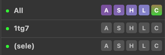
Next to the object names the menu, items are located. These are labelled A, S, H, L, C. These letters stand for Action, Show, Hide, Label, and Color. Go ahead and click a letter and observe the menu appearing. We will explore these menus in more detail later.
1.2 Molecular representations
PyMOL provides multiple molecular representations for visualization. For a quick overview of these use the main menu and click
1.2.1 Wizard → Demo → Representation
You can also find the wizard tools in the next to the mouse button. This will display the 8 different molecular representations available in PyMOL. These are lines, sticks, spheres, surface, mesh, dots, ribbon, and cartoon. Of these, the lines, sticks and cartoon representation are probably the most commonly used to display biomolecular structures. Go ahead and select various other demos from the menu on the right-hand side (e.g. Cartoon Ribbons). Click the End Demonstration button when you are done.
2 Exploring E. coli beta-galactosidase
2.1 Loading your first protein structure
In this tutorial we will first explore the structure of beta-galactosidase (LacZ) and investigate the molecular interactions with the inhibitor PETG – a cell permeable inhibitor.
To load the LacZ PDB structure into PyMOL, navigate in the main menu system:
File → Get PDB.. → [enter the 4-character PDB code 5a1a]
The PyMOL display panel will now show the 3D structure of E. coliLacZ in the default cartoon representation with the ligand shown as sticks colored by atom type. Note that the object panel now contains an entry named 5a1a representing our newly created object.
Familiarize yourself with the mouse controls before we move on:
Rotate: Press and hold the left mouse button while moving the mouse.
Zoom: Press and hold the right mouse button while moving the mouse.
Translate: Press and hold the middle mouse button while moving the mouse.
Clip the view: Scroll.
Click the Zoom button in the to zoom on all or selected molecules. The Orient button will orient the view to display the molecule along its longest axis aligned with the x-axis. (Try it out).
2.2 Using the visualization presets
PyMOL comes with multiple built-in visualization preset views. These can be accessed through the Action (A) button(s) in the object panel. Click the A next to the 5a1a object. From the menu that appears click preset → ligands. The program will now automatically zoom into the ligand region of the protein. In our case the protein is a tetramer and binds four ligands, so we zoom to see all four. To see individual ligands use the "Zoom" button in the and choose “Next Ligand”, which will zoom to a view of an individual ligand.
Observe that there was a change in the representation of the protein to ribbon, the residues close to the ligand will show in lines, and the ligand is shown as sticks. Also notice the yellow dashed lines appearing between polar groups between the protein and ligand (Figure 2).
PyMOL also offers various similar visualization presets for the protein-ligand interactions. Explore these through navigating in the object panel (A → preset → ligand sites). See in particular the following:
cartoon: provides the same view as ligands but with the protein in cartoon representation,
solid surface: draws the binding pocket in solid surface,
transparent: draws the binding pocket in transparent surface.
2.3 Displaying molecular representations
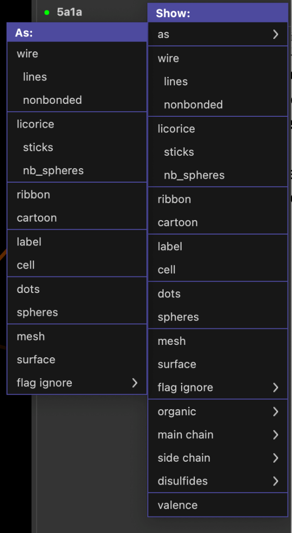
Besides the various automatic representation presets shown above you can also set the molecular representation to be shown more manually. Click the S (show) button from the object panel next to the 5a1a entry. From the menu appearing you can choose to show various molecular representations, such as lines, sticks, ribbon, etc. From the first menu entry (as) you can select the representation in which you want the protein to be shown as.
Try the following and observe how the molecular representation changes in the viewer window:
S → as → spheres
S → as → lines
S → cartoon
Observe that using S → as changes the whole representation, whereas S → adds a representation on top of the former representation.
The various representations can also be hidden using the H (hide) button from the object menu. e.g. try the following:
H → cartoon
H → lines
Explore also the various other options in the Show menu (such as organic, main chain, etc).
Make sure you use S → as → lines before continuing to the next step.
2.4 Working with atom selections
More customized visualization and investigations of biomolecular structures often requires functionality to select individual or group of atoms. In PyMOL the simplest approach for atom selection is by simply clicking the particular atom in the display panel.
Click any atom in the protein. Note the new entry in the object menu on the right-hand side called (sele), and the selected atoms are shown in the display panel with small pink squares.
To zoom in on your selection simply do A → zoom on the (sele) entry.
You can now assign a different molecular representation to the selection e.g. with S → sticks on the (sele) entry. The selected atoms should now appear as sticks in display panel.
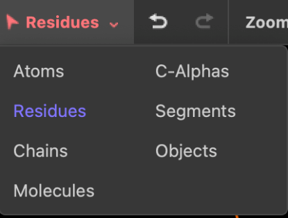
Even though we initially only clicked at one atom in the protein, all atoms in the residue are selected by default. This behavior can be changed by clicking on the "selection button" in the left side of the [top menu]{top-menu} (named "Residues" by default). If you choose Atoms, you will be able to select a single atom when clicking on it in the display panel. Now zoom out to see the full molecule using the Zoom button in the "top menu". If you choose Chains, you will be able to select one chain of the tetramer when clicking on it in the display panel. Choose Residues again before continuing.
The parenthesis in (sele) means that this entry is a selection. Conversely, the 5a1a entry is an object, and (sele) is an atom selection of this object. The selection entry has much the same menu system attached to it as an object entry.
Another way of selecting residues is through the "sequence viewer" which you can toggle on/off through the SEQ (for sequence) button in the . When clicking SEQ once you will see the "sequence viewer" on the top of the "display panel". To select a residue from here, simply click (and drag) the relevant residue codes. To disable the selection, click on an empty part in the display panel, or click the (sele) entry in the object menu.

Selections can be deleted by clicking A → delete selection, and renamed with A → rename selection.
2.5 Color the atom selections
With selections we can easily color different elements in the structure. As an example, select a part of the protein, then use the C button (for color) next to the selection to change the color e.g. from green to blue.
Note that it is often useful to color by atom elements, i.e. to keep oxygens red, nitrogens blue, sulphurs yellow etc, and only adjust the colors of carbon atoms. This coloring option is available through C → by element → CHNOS.
Task: Based on the tools shown so far, try and select the 4 chains of the LacZ, and color them 4 different colors
2.6 Overview of LacZ
In the following we will focus on the monomer to make a nice figure for the interaction between LacZ and PETG (named PTQ in the model). With our selection skills from above we can now easily create a nice overview figure of E. coli LacZ in complex with PTQ.
Start by focusing on the entire protein by clicking on the Orient button.
Show LacZ as lines by using S → lines and show the ligand PTQ as spheres by using S → organic → spheres.
Now use the mouse to select the PTQ ligand in one of the subunits and name the selection "PTQ". In the same subunit, click the protein and rename the selection "protein".
To hide the other subunits, use (protein) → H → unselected and the show the ligand again using (PTQ) → S → spheres.
Now use Zoom → Visible to focus on the chosen subunit.
2.6.1 Cartoon representation
Show the protein selection in cartoon representation. Try different coloring options for the two selections and find a suitable orientation that shows the ligand binding site.
Make sure to color the ligand with different atom colors and with a color for the carbon atoms that makes it stand out using (PTQ) → C → by element → CHNOS.
Color the protein by secondary structure elements (hint: C → by ss) to see which elements are close to the binding site.
Color the protein to identify N-terminal and C-terminal ends (hint: C → spectrum → rainbow) to see which parts of the protein are close to the binding site.
Color the protein in a more neural color to make the ligand stand out.
Save this session by navigating in the main menu before we continue: File → Save session.
Saving sessions allows you to save the precise way that your current setup looks, and not just the positions of atoms in the file, like with a pdb file.
2.6.2 Surface representation
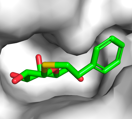
While the cartoon representation displays how the protein chain is folded, the surface representation is better for displaying cavities and other surface properties. From the show (S) menu of the protein selection entry, select surface and show the ligand as sticks. Color the protein in white and PTQ as green CHNOS. Zoom on the ligand using (PTQ) → A → zoom and observe the cavity in which PTQ binds, which should look like the image on the right. Save it as a session file.
Verify that you still have the selections (protein) and (PTQ) in the object menu on the right. Click Zoom → Visible and show the protein as cartoon representation and PTQ as sticks.
2.7 Exploring the binding of PTQ
To explore the binding site in more detail it can be useful to only select and show the residues in the immediate vicinity of the ligand. This can be done by using the modify function from the action (A) menu:
Click on the ligand to make a new selection. From the selection entry click (sele) → A → modify → around → residues within 5 A. This approach will modify the selection to contain the atoms around the ligand (and not the ligand itself). Rename this selection to near using A → rename selection. Our new (near) selection contains the atoms within 5 Å of the ligand. Show these residues as lines using (near) → S → lines and show waters and ions as non-bonded spheres using (near) → S → nb_spheres. Zoom on the selection using (near) → A → zoom.
Now that we see all residues close to the ligand, we can more easily pick out residues particularly important for the binding of PTQ to LacZ.
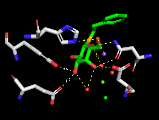
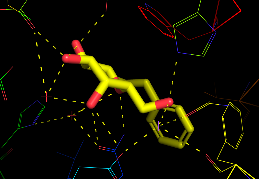
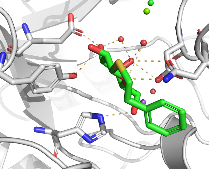
To show potential hydrogen bonds use (PTQ) → A → find → polar contacts → to other atoms in object. Select the residues that are in contact with the ligand by clicking on them one at the time. Rename the selection to hbondres. Use your skills from above to hide the protein and show the selected residues as sticks. Should look something like the image on the right.
You can use the measurement tool to measure the length of the polar contacts. Do this by clicking the wizard button in the or by navigating in the main menu through Wizard → Measurement. Follow the instructions on the screen (click first atom, click second atom). Notice the label with the distance (in Å), as well as a new measure01 object appearing in the object menu. Measure the distances between a few of the potential hydrogen bonds between PTQ and the protein residues (in particular the charged residues).
3 Publication quality figures for your report
3.1 Ray tracing for better resolution
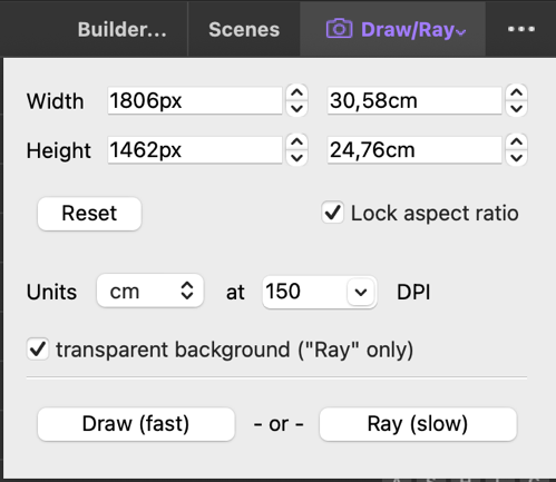
Now we’re getting close to a nice representation of the LacZ:PTQ complex. To use the figure in a publication (or report) it is good practice to enhance the quality and resolution by ray tracing.
Use the "Draw/Ray" button in the to make a ray tracing of your current view. Click "Ray (slow)" and observe the better quality when the ray tracing has completed.
3.2 Adjusting the default settings
For publications or reports in particular it’s good practice to use white background. Set this in the main menu by clicking Display → Background → White.
Personal preference obviously plays a role, but here are some additional settings that can be used to make a nice publication quality figure.
Setting → Cartoon → Fancy Helices
Setting → Rendering → Shadows → Medium
An example of a rendering is shown to the right.
Task: Use your new skills to color the protein, ligand and a few selected residues and display them in a nice view. Use your favorite ray trace mode and ray trace your view. Finally, you may want to annotate your image with amino acid names and numbers.
3.3 Some useful links
The internet is full of tricks on how to make nice figures with PyMOL. Here are some links that you might want to check out: